Implementing a MATLAB digital filter or controllers in C++
Controllers and filters are often a good way to stabilise a system, condition a signal or make a system follow a reference. The usual approach is to model the system or signal in an application like MATLAB and then design a filter or controller. Either by applying design rules, some sort of optimisation algorithm or tuning parameters experimentally. When the design is finished the controller or filter is not ready for use yet. It is still necessary to realise it in practice. This is often done digitally on a micro controller or real-time computer. This article will describe a effective, open and fast approach to realising a filter or controller in C++.
See also the post about a more generic filtering and control library.
We assume a Linear Time Invariant (LTI) continuous time transfer function of any order. If the transfer function is already discrete, you can skip the discretisation section.
Transfer function discretisation
Discretisation only applies when the controller of filter has been designed in continuous time. As the micro-controller can only execute computations as a sequence of discrete steps it is necessary to convert the continuous time transfer-function to a discrete time approximation. Different methods exist for converting a continuous time transfer function to a digital approximation. We will use the Tustin-approximation as it yields the best match in the frequency domain between the continuous and discrete time transfers.
The sample time \(T_s\) or frequency \(f_s = 1/Ts\) has to be determined. Faster sampling means a better approximation of the continuous time transfer-function. It will however require more computational power and performance of the Analog Digital Converter (ADC) input and Digital Analog Converter (DAC) / Pulse Width Modulation (PWM) outputs in terms of sampling frequency and noise. As a rule of thumb, select the sample frequency one or two orders of magnitude (10x – 100x) higher than the highest bandwidth that has to be controlled or filtered. For example, for a controlled pendulum with target bandwidth of 100 rad/s (16 Hz) select sample frequency 160 Hz or higher.
MATLAB provides tools for applying the Tustin-transformation to a continuous time transfer function. This is the continuous-to-digital c2d function. Assuming a transfer-function H, converting goes as follows:
Ts = 1e-3; % 1 ms sample time
Hd = c2d( H, Ts, 'tustin' );
Example: discretising a 5th order analog Butterworth filter
A 5th order analog Butterworth Low-pass filter is designed and discretised. The resulting and original transfer functions are compared in a bode diagram and step-response.
n = 5;    % Filter Order
f = 1e2;  % Cut-off frequency, Hz

[z,p,k] = butter(n,2*pi*f,'s');
[b,a]   = zp2tf(z,p,k);
H       = tf(b,a);

fs      = 1e3;
Hd      = c2d( H, 1/fs, 'tustin' );

figure(1);
h = bodeplot( H, Hd );
setoptions(h,'PhaseMatching', 'on', 'PhaseMatchingValue', 0);
bode( H, Hd );
figure(2);
step( H, Hd );
The resulting bode figure looks as follows:
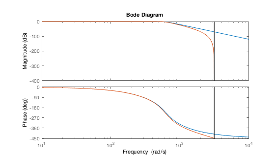
It is clear that the filter stops working at the Nyquist frequency \(F_s/2\). Up to 2e3 rad/s the discretised filter resembles great similarity with the original filter. It attenuates more than the original filter as the frequency is increased.
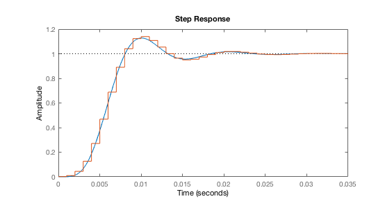
The step-response shows very good similarity between the original and the discretised filter. MATLAB shows how the discrete samples as a stair-signal.
The biquad filter as building brick
It is risky to implement complex controllers on digital hardware as round off errors might render the filter unstable. The biquad however is a very simple digital filter which can be proven being stable even if it is cascaded. Converting a filter to a series of biquads is the key to successful digital filter implementation.
Biquad stands short for bi-quadratic: its transfer function is the ratio of two quadratic functions in the z-domain (discrete time).
\[H(z) = \frac{b_0 + b_1z^{-1} + b_2z^{-2}}{a_0+a_1z^{-1}+a_2z^{-2}}\]By dividing both numerator and denominator by \(a_0\) the effective number of parameters is reduced to 5. If you are not interested in the filter details, you could go straight to the next section about converting filters to a series of biquads.
Direct form I
Finding the output of the filter for a sequence of input values is done by rearranging the equation \(y/u = H(z)\). This is visualized in the following figure:

Working from output back the following equation can be deduced:
\[y = b_0x+b_1xz^{-1} + b_2xz^{-2} - a_1yz^{-1} - a_2yz^{-2}\]This is called direct form I and is the most straightforward structure. It requires four memory elements. Two for the input (u) and two for the output (y) values. By rearranging this can be improved a bit.
Direct form II
Rearranging the equation reduces the memory usage by two elements without losing precision or performance. This is direct form II and it will be used in the following C++ implementation.

When the equation is worked out it looks as follows:
\[y = b_0w + b_1wz^{-1} + b_2wz^{-2}\]with
\[w=x-a_1wz^{-1}-a_2wz^{-2}\]Working this out shows that it is equivalent to the first form.
Converting the filter to a series of biquads
Biquads are also called Second Order Sections (SOS). MATLAB contains functions for converting arbitrary filter types to second order sections. This is done by rearranging all poles and zeros and grouping them into second-order sections (biquads). Depending on the filter type suitable functions are tf2sos, ss2sos, etc.
Example: converting a digital filter to biquads
Continuing to work on the previously created Butterworth low-pass filter. The function to convert transfer-functions to biquads has numerator (b) and denominator (a) coefficients as input. These can be obtained from a transfer-function object in MATLAB as follows.
sos = tf2sos( Hd.num{:}, Hd.den{:} );
The resulting matrix SOS looks as follows:
0.0011    0.0011         0    1.0000   -0.5219         0
    1.0000    2.0018    1.0018    1.0000   -1.1217    0.3674
    1.0000    1.9993    0.9993    1.0000   -1.3943    0.6996
The rows correspond to biquad sections, the columns correspond to respectively b0, b1, b2, a0, a1 and a2. Note that the coefficients have already been normalised.
C++ BiQuad implementation
The BiQuad class will store the five coefficients and two memory values. The storage footprint will thus be seven times the base type of storage. The BiQuadChain class will store pointers to BiQuad instances in a C++ std::vector.
The code can be found on GitHub. The following example application explains how to use the classes.
#include <cstdlib>
#include <iostream>
#include <iomanip>
#include <complex>
#include "BiQuad.h"

int main()
{

    BiQuadChain bqc;

    // Filter consists of two biquad sections
    BiQuad bq1( 4.82434e-03, 9.64869e-03, 4.82434e-03, -1.04860e+00, 2.96140e-01 );
    BiQuad bq2( 1.00000e+00, 2.00000e+00, 1.00000e+00, -1.32091e+00, 6.32739e-01 );

    // Add the biquads to the chain
    bqc.add( &bq1 ).add( &bq2 );

    // Find the poles of the filter
    std::vector< std::complex<double> > poles = bqc.poles();
    std::cout << "Filter poles" << std::endl;
    for( int i = 0; i < poles.size(); i++ )
        std::cout << poles[i] << std::endl;

    // Output the step-response of 20 samples
    std::cout << "Step response 20 samples" << std::endl;
    for( int i = 0; i < 20; i++ )
        std::cout << bqc.step( 1.0 ) << std::endl;

    // Done
    return EXIT_SUCCESS;

}
Generating the code for the filter directly from MATLAB is easy. Try the following snippet that takes a set of biquads sos.
i = 0;
for s = sos.'
    i = i + 1;
    fprintf('BiQuad bq%d( %.5e, %.5e, %.5e, %.5e, %.5e );\n', i, s(1), s(2), s(3), s(5), s(6));
end
fprintf('\nbqc');
i = 0;
for s = sos.'
    i = i + 1;
    fprintf('.add( &bq%d )', i);
end
fprintf(';\n');