Random Midpoint Displacement Fractal (RMDF)
The Random Midpoint Displacement Fractal (RMDF) is a fractal this is often used for generating height-maps, landscapes, rough surfaces and more. Its implementation is simple but the results are interesting, especially when a nice color-map is applied to the matrix and it is shown as a 3D-surface.

This specific implementation uses a simple linear congruential generator for producing pseudo random numbers. It is fast enough to generate the millions of random numbers required to generate the fractal in under a second. MATLAB image filtering functions are used for a number of computations because these functions are very efficient and allow for GPU utilization and parallelisation.
Implementation
The essence of the algorithm is to calculate midpoints of existing elements and adding random numbers of a distribution to them. Therefore it is called random-midpoint displacement fractal (RMDF).
The algorithm starts off with a 2×2 matrix containing four normal distributed random values with variance 𝛔² and a roughness value R in between 0 and 1 that influences the perceived roughness of the generated surface. The variance of the distribution decreases over time.
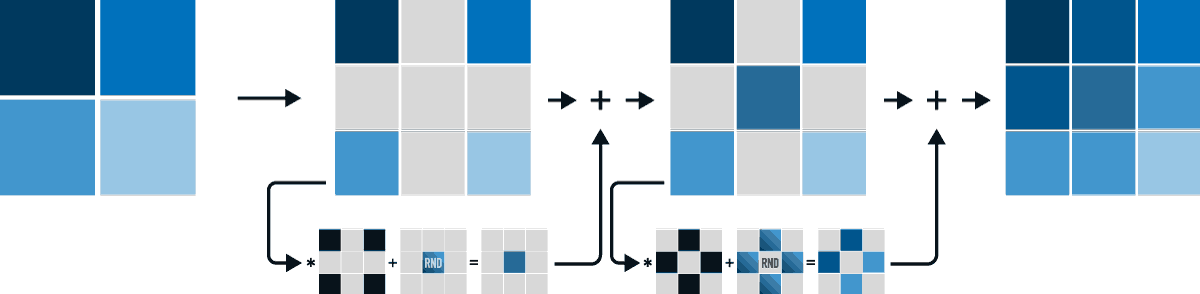
It is now time to find the midpoints and displacement them. One could calculate all midpoints and add a random number but this is not very fast. A smarter way would be to use convolutions. Two 2D kernels are created: A 3×3 kernel with value 1/4 in it’s corners, the rest zero; A 3×3 kernel with value 1/4 in top and bottom centre, and left and right center, the rest zero. This is shown in the figure below. The sum of the elements of the kernels is one, preserving the sum of the elements of the matrix that the kernel is convolved on.

An iteration of the algorithm is as follows:
- Reduce the variance of the random distributed pseudo random number generator: 𝛔² = R𝛔².
- Create a (2N-1)x(2N-1) zero-matrix and map every element of the NxN matrix to the new matrix as shown in the figure below.
- Convolve the diagonal kernel to the image, add random values to the resulting non-zero elements. Add the matrix element-wise to the original matrix.
- Reduce the variance of the random distributed pseudo random number generator: 𝛔² = R𝛔².
- Convolve the cross kernel to the image, add random values to the non-zero elements. Add the matrix element-wise to the original image.
The convolution with the diagonal kernel can be implemented as two sequential convolutions with 1D kernels as the kernel is separable ( rank(K) = 1 ). I trusted MATLAB to figure out the best way to apply the convolution by using the IMFILTER function. This function automatically checks for separability.
Performance
Timed execution shows that currently most of the time is spent calculating random numbers using the custom pseudo-random number generator.
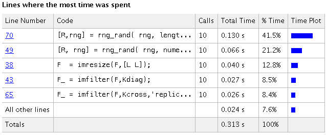
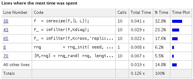
By replacing the custom PRNG with MATLAB’s built-in functionality a speed-up can be achieved.
Usage and Source-code
See the code on GitHub and generate a RMDF in seconds. The code is Octave compatible so you could use it for free. Note that you have to install and load the image package yourself.
pkg install -forge image
pkg load image
example

Sponsored content